Solving a system of Ordinary Differential Equations (ODEs)#
If you are not yet familiar with solving single ODEs with TFC, it is recommended you learn more about it via the ODE TFC notebook.
Consider the system of ODEs,
where a double dot over the variable indicates the second derivative with respect to time, subject to the boundary constraints
on the domain \(t\in[0,3]\). The analytical solutions to these differntial equations are:
To begin, let’s create the univariate TFC class and create the analytical solution so we can compare against it later.
[1]:
import jax.numpy as np
from tfc import utfc

# Create the univariate TFC class
N = 100 # Number of points in the domain
m = 19 # Degree of basis function expansion
nC = 2 # Indicates which basis functions need to be removed from the expansion

myTfc = utfc(N,nC,m,x0=0,xf=3,basis="LeP")

# Create the analytical solutions
yReal = np.vectorize(lambda t: -np.exp(2.0*t))
zReal = np.vectorize(lambda t: np.exp(2.0*t))
The next step is to develop the constrained expressions,
where \(g^y(t)\) is the free function for the \(y\) constrained expression and \(g^z(t)\) is the free function for the \(z\) constrained expression. In Python, we will use the Legendre orthogonal polynomials as the free function, \(g(t)\), so we will use the same \(g(t)\) function for each constrained expression, and pass in different unknowns.
[2]:
t = myTfc.x # Collocation points from the TFC class

# Get the basis functions from the TFC class
H = myTfc.H

# Create the constrained expressions
g = lambda t,xi: np.dot(H(t),xi)
y = lambda t,xi_y: g(t,xi_y) + ((3.0-t)/3.0) * (-1.0 - g(np.zeros_like(t),xi_y)) + t/3.0 * (-np.exp(6.0)-g(3.0*np.ones_like(t),xi_y))
z = lambda t,xi_z: g(t,xi_z) + ((3.0-t)/3.0) * (1.0 - g(np.zeros_like(t),xi_z)) + t/3.0 * (np.exp(6.0)-g(3.0*np.ones_like(t),xi_z))
This system of differential equations is linear, so we will use the same LS function to minimize the residuals of the differential equations. For systems of differential equations, we have multiple sets of unknowns–two in this case, xi_y and xi_z. Moreover, we have multiple residuals–again, two in this case. Therefore, we will combine the unknowns into a TFCDict and the residuals into a single function using hstack. The TFCDict functions much like a typically Python
dictionary, but with a few operations overloaded that allow it to be used by the LS and NLLS optimization routines. Moreover, it is registered as a known JAX type, so we can differentiate with respect to it if need be, much like a normal Python dictionary.
Although this system is linear, the same procedure should be followed for a nonlinear system of differential equations; the only difference is that the NLLS function should be used in place of the LS function: see the complex, nonlinear equations in the natural balloon shape probelms of Carl Leake’s dissertation (chapter 4) for more details.
[3]:
from tfc.utils import egrad, LS, TFCDict

# Create a TFCDict of the unknowns
xi0 = TFCDict({
    "xi_y": np.zeros(H(t).shape[1]),
    "xi_z": np.zeros(H(t).shape[1])
})

# Create the individual residuals
d2z = egrad(egrad(z))
d2y = egrad(egrad(y))

Ly = lambda t,xi: -d2y(t,xi["xi_y"]) - 4.0 * z(t,xi["xi_z"])
Lz = lambda t,xi: -d2z(t,xi["xi_z"]) + 8.0 * z(t,xi["xi_z"]) + 4.0 * y(t,xi["xi_y"])

# Combine the residuals into one function
L = lambda xi: np.hstack([Ly(t,xi), Lz(t,xi)])

# Minimize the residual using least-squares
xi,time = LS(xi0,L,timer=True)
Note that the last line in the above code block calls the JIT. Therefore, it may take a few seconds to run, because code is being compiled. However, once the code is finished compiling it runs very fast. The time returned by the LS function is the time it takes the compiled code to run, not the time it takes to compile the code itself. For more information on this function (and an associated class form) see the tutorial on LS.
Finally, lets compare the results to the true solution on a test set, and show some statistics about the TFC solution.
[4]:
# Calculate the error on the test set
t_test = np.linspace(0.0, 3.0, 100)
errY = y(t_test,xi["xi_y"]) - yReal(t_test)
errZ = z(t_test,xi["xi_z"]) - zReal(t_test)

# Print out the results
print(f"Run time: {time}")
print(f"Maximum error on y: {np.max(np.abs(errY))}")
print(f"Maximum error on z: {np.max(np.abs(errY))}")

# Plot the results
from tfc.utils import MakePlot

# This line is added for Python notebooks but is not necessary in a regular Python script.
%matplotlib inline
import matplotlib
matplotlib

p = MakePlot([r"$t$",r"$t$"],[r"$y$",r"$z$"])
p.ax[0].plot(t_test,y(t_test,xi["xi_y"]),label="TFC solution",color="c",linewidth=3)
p.ax[0].plot(t_test,yReal(t_test),label="Real solution",color="m",linestyle=":",linewidth=3)
p.ax[1].plot(t_test,z(t_test,xi["xi_z"]),label="TFC solution",color="c",linewidth=3)
p.ax[1].plot(t_test,zReal(t_test),label="Real solution",color="m",linestyle=":",linewidth=3)
for ax in p.ax:
    ax.legend()
    ax.grid()
p.PartScreen(6,8)
p.fig.tight_layout(w_pad=None)
p.show()
Run time: 0.0008738219999999686
Maximum error on y: 2.1866952693017083e-12
Maximum error on z: 2.1866952693017083e-12
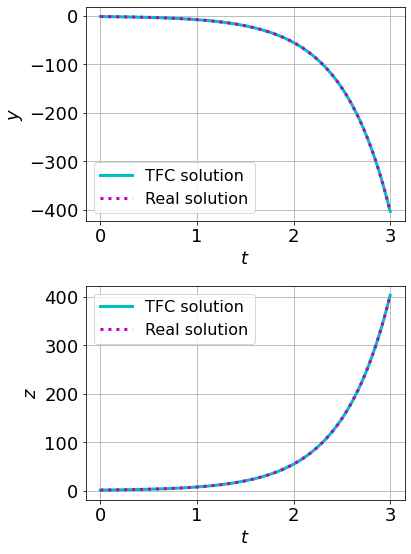
The difference between the TFC estimated solution and real solution is on the order of \(10^{-12}\), and the TFC solution was obtained in less than a thousandth of a second.