Nonlinear Least Squares#
This notebook discusses and explains how to use the nonlinear least squares function, NLLS, and the nonlinear least squares class, NllsClass, available from the TFC utilities. They are used regularly in the context of TFC when minimizing the residual of differential equations, but are written in a general way so that they can be applied to any problem that requires nonlinear least-squares.
The NLLS function and NllsClass can utilize automatic differentiation, so the user need only supply the residual function. Moreover, both are designed to work with unkowns given as an array, a TFCDict, or a TFCRobustDict; the latter two options in particular are extremely useful when one has multiple arrays of unkowns such as in systems of ODEs or PDEs. Moreover, both NLLS and NllsClass JIT the entire nonlinear least-squares process, and provide the option to calculate
the run-time of the compiled code.
NLLS Function#
The NLLS function is designed for cases where the nonlinear least-squares needs to be run only once.
Positional input arguments#
This function function takes in two required positional arguments and one optional position argument. The two required positional arguments are the initial guess for the unknowns and the residual function: the residual function must be structured such that the unkowns are the first argument. The one optional position argument is *args, which is used if the residual function has more arguments than the unknowns. In other words, the residual function should be of the form, \(\mathbb{L}(\xi,*args)\), where \(\mathbb{L}\) is the residual function, \(\xi\) are the unknowns, and *args are any additional arguments.
Optional input keyword arguments#
The optional keyword arguments to the NLLS function are:
\(\mathcal{J}\) - User-specified Jacobian. The default option is to compute the Jacobian of \(\mathbb{L}\) with respect to \(\xi\) using the automatic differentiation
tol - Tolerance used in termination criteria. Default is \(1\times10^{-13}\).
maxIter - Maximum number of nonlinear least-squares iterations. Default is 50.
User specified condition function. Default is None, which results in a condition that checks the three conditions listed in termination criteria.
body - User specified body function. Default is None, which results in a body function that performs least-squares using the method provided and updates \(\xi\), \(\Delta \xi\) and \(it\), the current number of iterations.
timer - Setting this to True will time the nonlinear least squares using the timer specified by timerType. The default is False.
timerType - The timer from the timer package that will be used to time the code. The default is process_time.
printOut - Setting this to true enables printing. The printout is the iteration number and value of \(\max(|\mathbb{L}|)\) at each iteration.
printOutEnd - Sets the end keyword argument in print used by printOut. Default is “\n”
method - Method used to invert the matrix at each iteration. The default is pinv. The two options are:
pinv - Uses Numpy’s pinv to perform the inversion.
lstsq - Uses Numpy’s lstsq to perform the inversion.
Outputs#
The outputs of the function are:
\(\xi\) - The value of \(\xi\) at the end of the nonlinear least squares.
\(it\) - The number of iterations.
time - If the keyword argument timer = True, then the third output is the time the nonlinear least-squares took; otherwise, there is no third output.
Termination criteria#
The NLLS function stops iterating when any of the following criteria are true:
\(\max(|\mathbb{L}|) < \verb"tol"\)
\(\max(|\Delta \xi|) < \verb"tol"\)
Number of iterations >
maxIter
As a demonstrative example, suppose one wanted to approximate the function \(y = a e^{b x}\) using a linear expansion of Chebyshev polynomials, where the coefficients in that expansion are nonlinear combinations of a paramter \(\xi\).
[1]:
import jax.numpy as np
from tfc.utils import BF, NLLS, MakePlot

# This line is added for Python notebooks but is not necessary in a regular Python script.
%matplotlib inline

# Create the true data
a = 1/3
b = 2
x = np.linspace(0,1,101)
y = a*np.exp(b*x)

# Create the Chebyshev polynomials
cp = BF.CP(0.,1.,np.array([-1],dtype=np.int32),20)
H = cp.H(x,0,True)

# Create the approximating function
g = lambda xi: np.dot(H,xi**2-xi)

# Create the residual function
L = lambda xi: g(xi)-y

# Solve for the unknowns using NLLS
xi0 = np.zeros(H.shape[1])
xi,it,time = NLLS(xi0,L,timer=True)

# Plot and print results
p = MakePlot('x','y')
p.ax[0].scatter(x[::10],y[::10],color='r',label='True data',zorder=3)
p.ax[0].plot(x,g(xi),'b-',label='NLLS Approximation')
p.ax[0].legend()
p.show()

print("NLLS run time: "+str(time)+" seconds.")
print("Maximum error: "+str(np.max(np.abs(L(xi)))))
NLLS run time: 0.0017242620000001985 seconds.
Maximum error: 4.996003610813204e-16
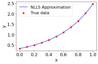
As one can see, parameters \(\xi\) were found in a matter of milliseconds that reduce the maximum residual value to nearly machine level precision. As mentioned earlier, this can be done not just for arrays of unkowns, but TFCDicts and TFCRobustDicts as well. In addition, the loss functions can take extra arguments other than the unknown parameters. For example, suppose we have a dictionary of unknowns used in our approximating function \(g\), and that \(g\) also takes in
some other arguments.
[2]:
from tfc.utils import TFCDict

# Create the approximating function
g = lambda xi,c1,c2: c1*np.dot(H,xi['xi1']*xi['xi2']-xi['xi2'])+c2

# Create the residual function
c1 = 2.
c2 = 1.
L = lambda xi,c1,c2: g(xi,c1,c2)-y

# Solve for the unknowns using NLLS
xi = TFCDict({'xi1':np.zeros(H.shape[1]),
              'xi2':np.zeros(H.shape[1])})
xi,it = NLLS(xi,L,c1,c2,printOut=True,tol=1e-15)

# Plot and print results
p = MakePlot('x','y')
p.ax[0].scatter(x[::10],y[::10],color='r',label='True data',zorder=3)
p.ax[0].plot(x,g(xi,c1,c2),'b-',label='NLLS Approximation')
p.ax[0].legend()
p.show()

print("Maximum error: "+str(np.max(np.abs(L(xi,c1,c2)))))
Iteration: 0    max(abs(res)): 2.6645352591003757e-15
Iteration: 1    max(abs(res)): 2.220446049250313e-16
Maximum error: 2.220446049250313e-16

Once again, \(\xi\) parameters were found that reduce the maximum residual value to nearly machine level precision.
Nonlinear least-squares class (NllsClass)#
The NllsClass is designed to be used when the nonlinear least-squares must be called multiple times. The class saves the JIT-ed nonlinear least-squares function which can be called via the run method, whereas the NLLS function just runs it once. The NllsClass is initialized in the same way the NLLS function is, except the *args positional argument is eliminated; The *args argument is only used when calling the run method. The run method only takes in the two position arguments
\(\xi\) and *args, and the outputs are the same as the NNLS outputs. To demonstrate, consider the previous example, but run in a for loop for different values of \(c_1\) and \(c_2\).
[3]:
import numpy as onp
from tfc.utils import NllsClass

# Create the NllsClass
nlls = NllsClass(xi,L,timer=True,tol=1e-15)

# Allocate memory
c1 = np.linspace(1,2,10)
c2 = np.linspace(0.5,1.5,10)
err = onp.zeros_like(c1)
time = onp.zeros_like(c2)
xi = TFCDict({'xi1':np.zeros(H.shape[1]),
              'xi2':np.zeros(H.shape[1])})

# Run the nonlinear least-squares for different values of c1 and c2
for k in range(c1.shape[0]):
    xi,it,time[k] = nlls.run(xi,c1[k],c2[k])
    err[k] = np.max(np.abs(L(xi,c1[k],c2[k])))

print("NLLS average run time: "+str(np.mean(time))+" seconds.")
print("Maximum error: "+str(np.max(err)))
NLLS average run time: 0.004411600800000049 seconds.
Maximum error: 8.881784197001252e-16
Once again, \(\xi\) parameters were found in a matter of milliseconds that reduce the maximum residual value to nearly machine level precision in each case.